An R package to visualise glm coefficients • prettyglm

Overview

prettyglm is an R package which provides a set of functions which create beautiful coefficient summaries of generalised linear models.

Installation

You can install the latest CRAN release with:

install.packages('prettyglm')

A Simple Example

To explore the functionality of prettyglm we will use a data set sourced from kaggle. To learn more about each of the provided functions please read the articles.

Pre-processing

A critical step for this package to work well is to set all categorical predictors as factors.

library(prettyglm)
library(dplyr)
data("bank")

# Easiest way to convert multiple columns to a factor.
columns_to_factor <- c('job',
                       'marital',
                       'education',
                       'default',
                       'housing',
                       'loan')
bank_data  <- bank_data  %>%
  dplyr::filter(loan != 'unknown') %>% 
  dplyr::filter(default != 'yes') %>% 
  dplyr::mutate(age = as.numeric(age)) %>% 
  dplyr::mutate_at(columns_to_factor, list(~factor(.))) %>% # multiple columns to factor
  dplyr::mutate(T_DEPOSIT = as.factor(base::ifelse(y=='yes',1,0))) #convert target to 0 and 1 for performance plots

Building a glm

For this example we will build a glm using stats::glm(), however prettyglm is working to support parsnip and workflow model objects which use the glm model engine.

deposit_model <- stats::glm(T_DEPOSIT ~ marital +
                                        default:loan +
                                        loan +
                                        age,
                             data = bank_data,
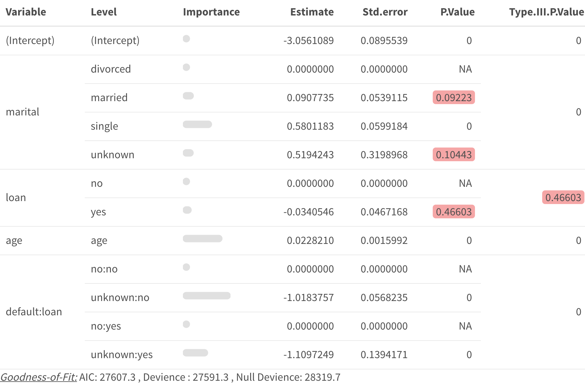
                             family = binomial)

Table of model coefficients

pretty_coefficients() creates a neat table of the model coefficients, see vignette("creating_pretty_coefficients").

pretty_coefficients(deposit_model, type_iii = 'Wald')

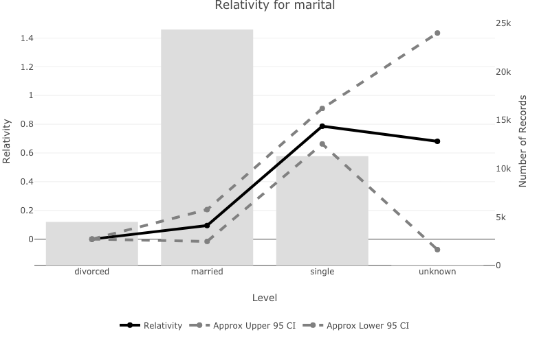
Create plots of the model coefficients

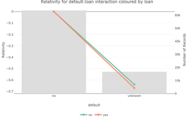
pretty_relativities() creates beautiful plots of model coefficients, see vignette("simple_pretty_relativities") and vignette("interaction_pretty_relativities") to get started.

job

pretty_relativities(feature_to_plot = 'marital',
                    model_object = deposit_model)

age

pretty_relativities(feature_to_plot = 'age',
                    model_object = deposit_model)

default:loan

pretty_relativities(feature_to_plot = 'default:loan',
                    model_object = deposit_model,
                    iteractionplottype = 'colour',
                    facetorcolourby = 'loan')

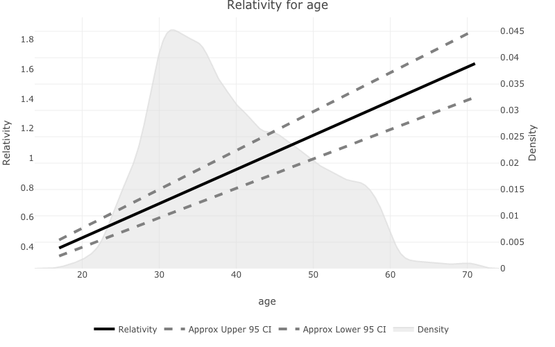
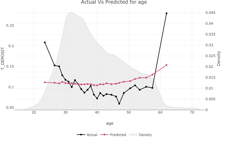
Visualising one-way model performance

one_way_ave() creates one-way model performance plots, see vignette("onewayave") to get started.

age

one_way_ave(feature_to_plot = 'age',
            model_object = deposit_model,
            target_variable = 'T_DEPOSIT',
            data_set = bank_data)

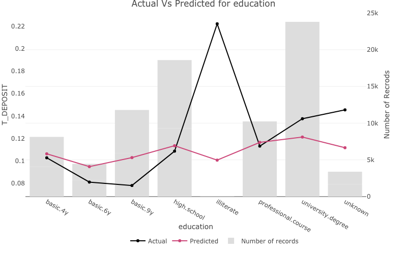
education

one_way_ave(feature_to_plot = 'education',
            model_object = deposit_model,
            target_variable = 'T_DEPOSIT',
            data_set = bank_data)

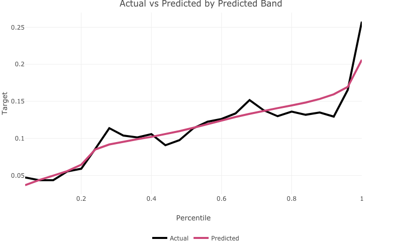
Visualising overall actual vs expected bucketed

actual_expected_bucketed() creates actual vs expected performance plots by predicted band, see vignette("visualisingoverallave") to get started.

actual_expected_bucketed(target_variable = 'T_DEPOSIT',
                         model_object = deposit_model)

prettyglm